
Lab Notes: Lock-In Detection
How to measure signals buried in noise

In Lab Notes, I describe what day-to-day life is like in a quantum/RF lab. In this first article, we’ll go into a workhorse of sensitive measurement: the lock-in amplifier.
One of the most useful techniques for precision measurement is the “lock-in” measurement. This is used when you send a known signal into a device (DUT — device under test) and want to see exactly what the system does to the signal. The problem is that quite often, the signal gets buried under noise as it makes its way through the DUT and other experimental apparatus, so how do you reliably extract it?
This is where the lock-in measurement comes in. The schematic below sets it up:
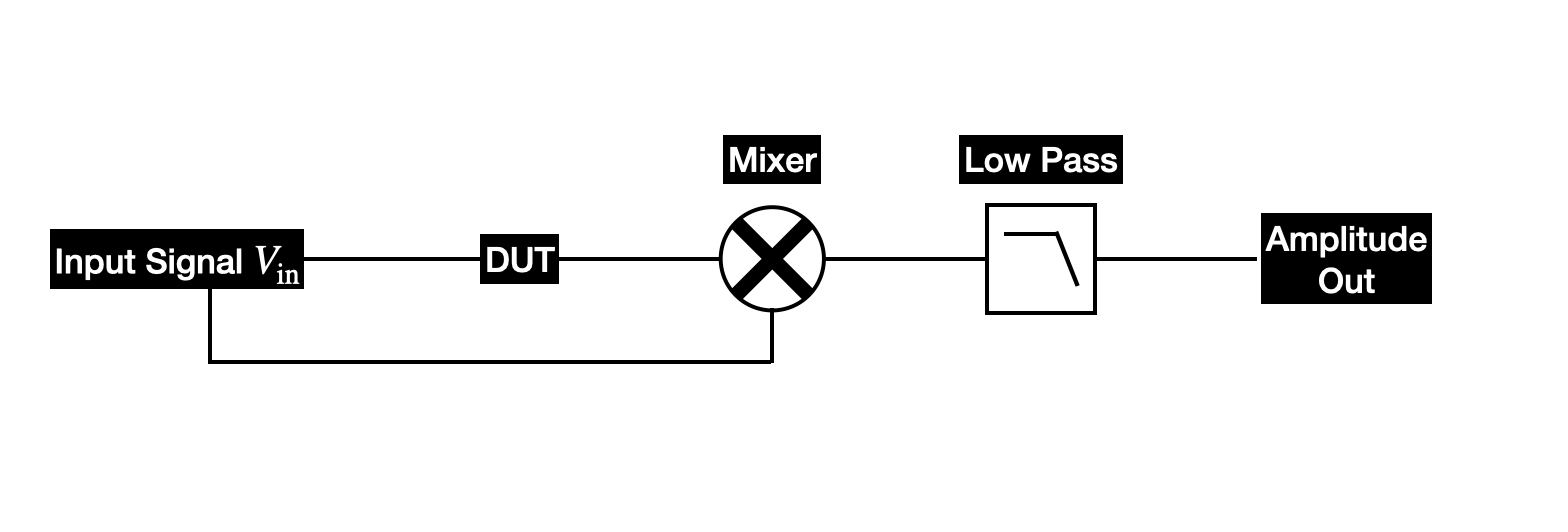
In a lock-in setup, you send a signal Vin to the DUT at a known frequency ω0, let’s say
After the DUT, your signal will change its amplitude and pick up some phase shift φ, which tells you about the physics of the system. For now, let’s assume it picks up 0 phase — we’ll deal with this later.
It will also generically pick up some noise n. Putting the contributions together, we get that the signal after the DUT is:
Let’s assume for simplicity that n(t) is white noise. This is a pretty common case in real life and means that it has equal power at all frequencies, i.e. it’s flat as a function of frequency.
So now our goal is to learn about the physics of the DUT by extracting A. How do we do this?
After the DUT, the output signal goes towards a device called a mixer. A mixer basically takes two input signals with frequencies ω1, ω2 and multiplies them together. In the lock-in setup, one of the mixer inputs is the output of the DUT. The other input is the original signal Vin we sent to the DUT in the first place:
Using trig identities (specifically cos(A+B) = cosAcosB - sinAsinB), you can show that
The first term here has a frequency of 2ω0 and the second term has a frequency of 0. Note that this zero frequency term is proportional to the amplitude of the signal after the DUT, which is all the information we need. Our goal therefore is to isolate this 0 frequency component.
The third term is white noise multiplied by a cosine at frequency ω0. It might look like this term ends up overall at frequency ω0 but this is actually not true. Like the original white noise, this “mixed noise” term also ends up being flat in frequency space.
Optional: Why is the noise term flat?
You could just believe me and move on — and indeed if you don’t like calculus you should — but I’m not going to miss an opportunity to take a Fourier transform so let’s see if we can at least motivate quantitatively why the noise term stays flat. Let’s compute the Fourier transform of n(t)cos(ω0 t):
Here, we’re using the convolution theorem which tells us how to take Fourier transforms of products. The Fourier transform of the product of two functions in the time domain is the convolution of their Fourier transforms in the frequency domain. The convolution integral is defined as
The Fourier transform of cos(ω0 t) is a standard result1
Let’s say that the Fourier transform of the noise function n(t) is N(ω). Then we want to take the convolution between N and the transform of the simple cosine. Chugging through the integral and using the properties of delta functions, you can show the convolution of the Fourier transforms ends up being proportional to
N(ω - ω0) is the original flat spectrum N just shifted by ω0 units right in frequency space and N(ω + ω0) is the original flat spectrum shifted left. So the final Fourier transform is the sum of two flat things in frequency space and hence will be flat also.
Visualising a Lock-In Measurement
Ok so now after the mixer we have a 2ω0 term, a 0 frequency term, and the flat noise term. We can see what’s happening so far pictorially. These plots show the noise power (technically the power spectral density) before and after the mixer on the y-axis vs frequency on x-axis.
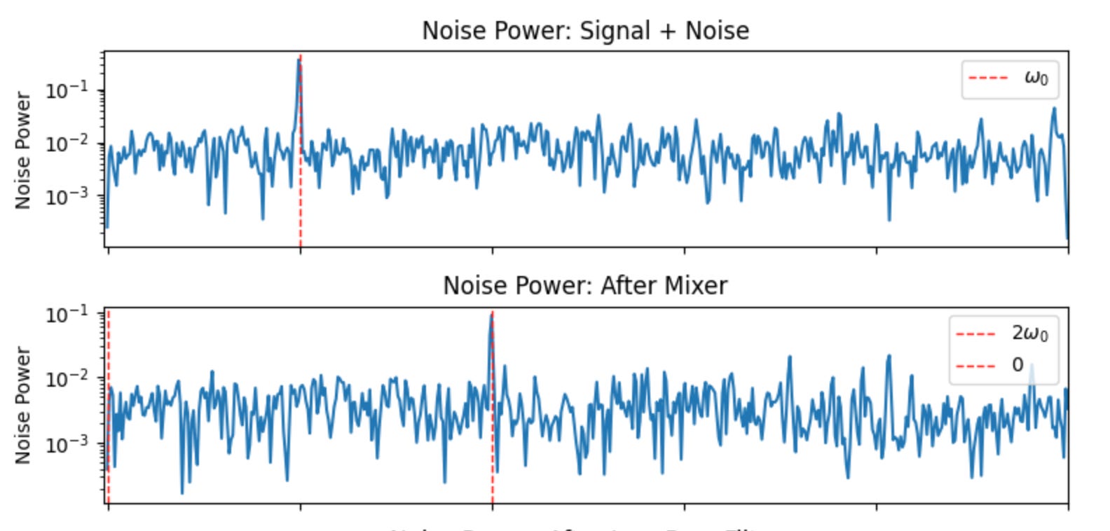
Before the mixer, we have our spike at ω0 representing the original signal plus all of the noise. After the mixer, we see that there is a spike now at 2ω0 and our critical component at 0, both sitting on the flat noise baseline.
Now we apply a low-pass filter (LPF), with an appropriate frequency cutoff to isolate the zero frequency component and kill the 2ω0 contribution. This is what the noise power looks like after a low-pass filter
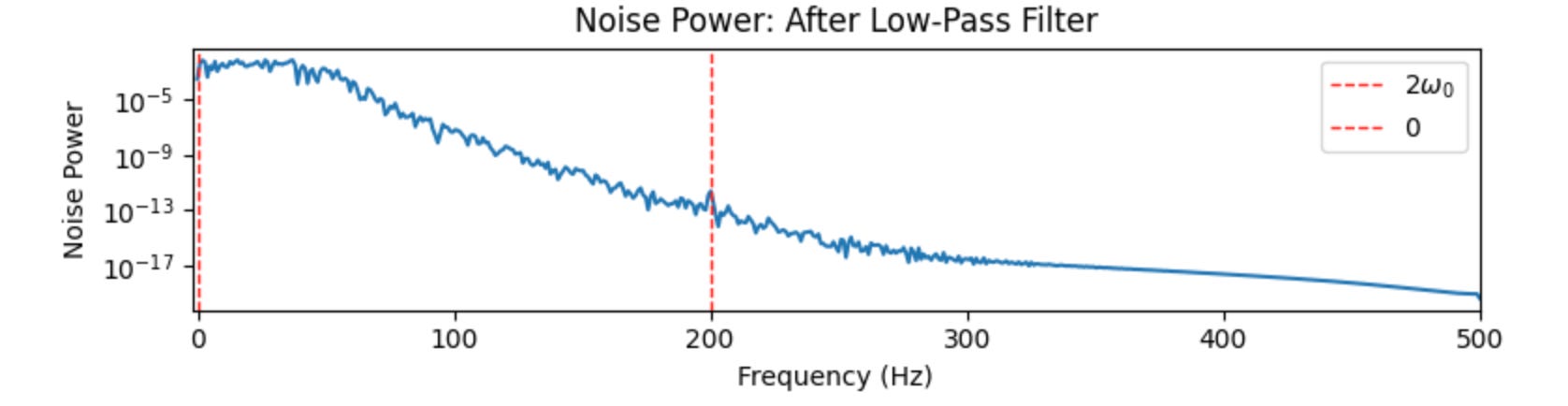
The power at 2ω0 is now ~10 orders of magnitude less than the power at zero frequency! This output is basically a zero frequency — also called DC for direct current — signal that is super easy to read out and measure with a voltmeter. Since this DC voltage is just proportional to the amplitude A, we are done.
FYI I wasn’t explicit about this but it’s called a lock-in measurement because you lock into the frequency of interest and use the mixer and LPF to isolate it.
Getting Amplitude and Phase
Earlier, I said we’re assuming that your DUT doesn’t cause any phase change on the input signal. That is obviously not true generally, so how do you modify the simple lock-in measurement I showed you to get both amplitude A and phase φ?
More concretely, while Vin stays the same, in this case, V_DUT is modified:
In the previous case, we ended up with one zero frequency voltage that was directly proportional to A. You can show that if you do the lock-in procedure we described above, the zero frequency voltage will be (A/2)cosφ. We have one equation but 2 variables to solve for, which is not going to work.
How do we introduce the extra equation? By using two mixers!
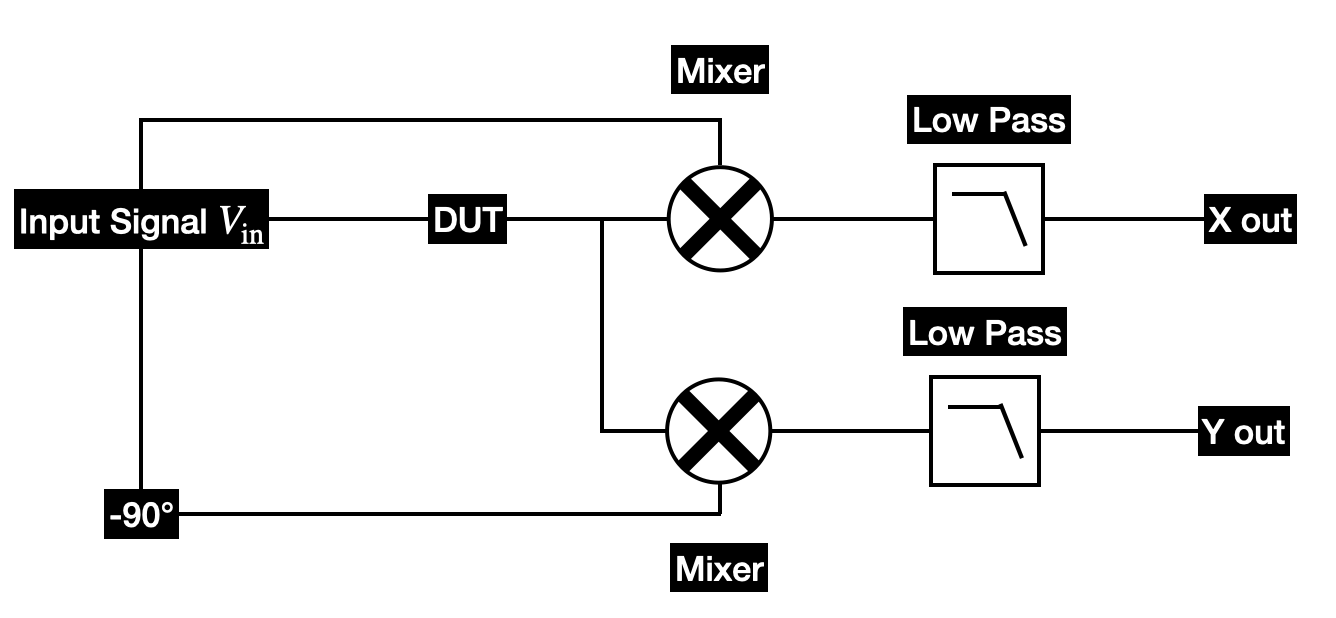
Now there are two outputs, one from each mixer, which we call X and Y. The reference input to the first mixer is still just Vin = cos ω0 t. The input to the second mixer is the original input with a 90 degree phase shift:
Both mixing processes now happen exactly the same with the same DUT signal — the only difference is their reference signals. The signals after both mixers are:
Now you put both signals through a low-pass filter to get the X and Y components of the signal:
Now that we have two equations, getting A and φ is trivial
Where atan2(x) is the modified arctangent function.
Terminology note: X and Y are called the quadratures of the signal being measured. They can also be referred to as I (in-phase) and Q (quadrature) respectively.
Lock-In Amplifiers
The lock-in method is a specific application of a more general technique called homodyne detection. In homodyne detection, we mix an input signal at a frequency ω with a reference signal also at the same frequency.
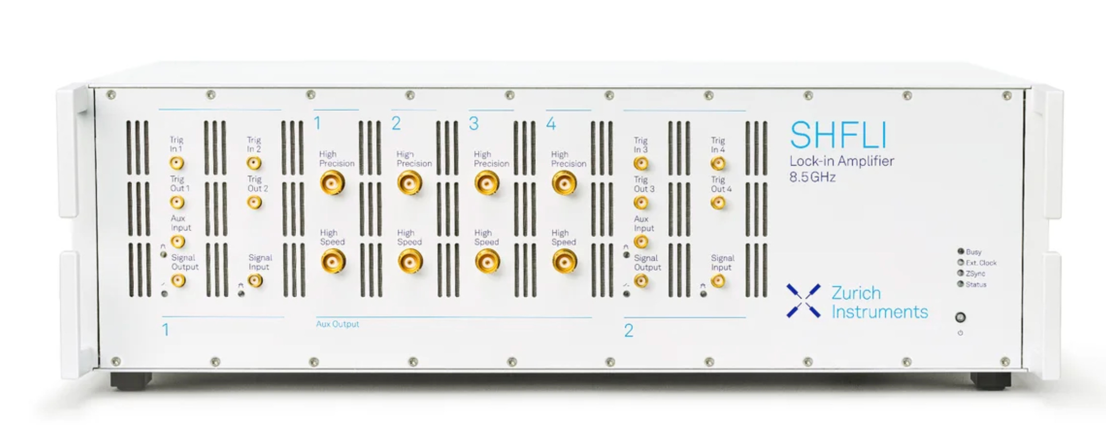
Lock-in measurements are so useful that many companies actually make dedicated lock-in amplifiers. One example we use in our lab is the Zurich Instruments SHFLI Lock-In Amp which works all the way up to 8.5 GHz, which is necessary since most superconducting quantum operation happens up in the GHz microwave range.
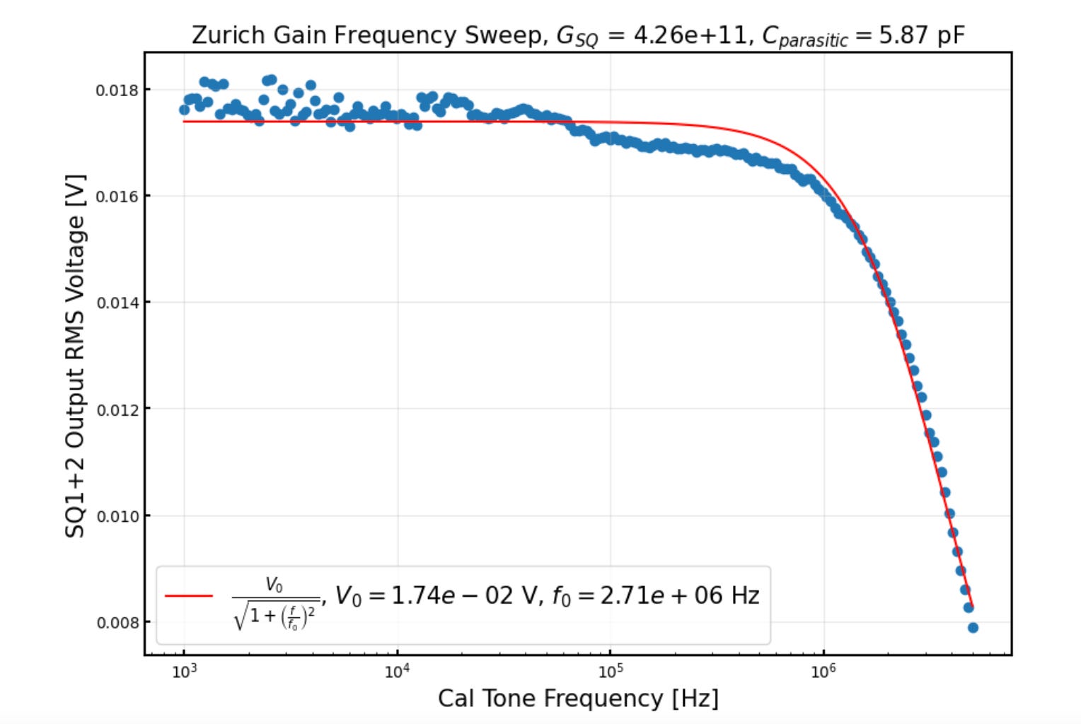
Lock-in measurements are super central to many precision measurements because they’re one of the most basic ways you characterise devices like qubits or amplifiers. One thing you quite often want to know is the gain of your amplifier, so the simplest thing to do is to connect the amplifier to the lock-in amplifier and sweep the frequency of the input signal. By measuring the output amplitude and phase as a function of frequency, you characterise the gain. Here is a plot I made for a rough calibration of a superconducting quantum interference device (SQUID) using one of the Zurich Instruments lock-in amplifiers.
Lock-in detection is involved in virtually every precision measurement in RF and quantum labs. By “locking in” on the chosen frequency, mixing it down to DC, and filtering away everything else, you can recover tiny signals buried under noise and even track their phase. Whether you’re characterising amplifier gain or reading out a superconducting qubit, the lock-in amplifier is a trusted workhorse.
I’m using the symmetric convention where the forward and reverse Fourier transforms have the same normalising factor 1/√(2π)